Mapping with Confidence: A Beginner’s Guide to Reference-Based Assembly

14 minute read

When you have a good reference genome, reference-based assembly is often the most efficient way to make sense of your sequencing data. In this post, we’ll walk through a hands-on example of mapping Illumina reads to a bacterial reference genome and calling variants.

A New Strain on the Bench

You’ve just isolated an E. coli strain from a patient sample. It grows like E. coli, but is it really just like the non-pathogenic E. coli K-12 MG1655 reference, or something else entirely? Let’s find out by mapping its DNA to the MG1655 reference genome.

Step 0: Setting up your Conda environment

Before we begin analyzing any data, we will create two different Conda environments that will be used during this tutorial. If you don’t have Conda installed on your system, please refer to this post for advantages of using a package manager and setting it up with some useful channels. I have also included versions that I used for this tutorial for reproducibility.

Tip: It’s often a good idea to create separate Conda environments for different applications. For example, sra-tools is only needed for downloading data and isn’t tightly connected to the downstream reference-based assembly workflow. By isolating it in its own environment, we keep our analysis environment (reference-assembly) clean, reproducible, and free from unnecessary dependencies. This also reduces the risk of version conflicts between tools.

Conda environment #1: sra-tools

This environment will use sra-tools to download sequencing data from NCBI’s Sequence Read Archive (SRA).

conda create -n sra-tools -y sra-tools=3.2.1

Conda environment #2: reference-assembly

This environment will use various tools that are commonly used during reference-based assemblies.

conda create -n reference-assembly -y \
  bcftools=1.21 \
  bwa-mem2=2.3 \
  fastp=1.0.1 \
  fastqc=0.12.1 \
  freebayes=1.3.10 \
  multiqc=1.30 \
  samtools=1.21 

Step 1: From Bench to FASTQs

In the lab, here’s what would have happened before you even saw any data:

DNA Extraction
The colony you isolated would be lysed, and its genomic DNA purified using a commercial kit or in-house protocol.
Library Preparation
The DNA would be fragmented (usually via enzymatic fragmentation or sonication), and sequencing adapters added. For Illumina sequencing, this usually also includes adding indexes (barcodes) to each sample that will allow multiplexing your samples to reduce the overall cost of sequencing per sample.
Sequencing
The prepared library would be loaded on a sequencer. The sequencer reads millions of DNA fragments simultaneously, producing paired-end reads if performing short-read sequencing (ex: 150 bp each, forward and reverse). More information can be found in this post.
FASTQ Delivery
The sequencing core facility would then send you the raw sequencing files, FASTQ files, containing your reads and their quality scores. This is where the bioinformatics begins.

Note: For this tutorial, instead of prepping DNA yourself, we’ll use public data from a previous study that were deposited in SRA. The Illumina short reads (SRA Accession ERR2138591) come from sample VREC1013, which was sequenced and described in this study by Decano et al. (2019).

First, we’ll download the Illumina reads from SRA:

# Activate the conda environment
conda activate sra-tools

# Download the run using the provided accession
prefetch ERR2138591

# Convert SRA format to FASTQ
fasterq-dump --split-files ERR2138591 -O ./raw_fastq

Tip: Use --split-files when using fasterq-dump with paired-end data so you get separate forward (_1.fastq) and reverse (_2.fastq) reads. Many tools expect this format.

Since we suspect our bacterial sample is E. coli, we’ll begin by using the well-established laboratory strain K-12 MG1655 as our reference genome (Accession GCF_000005845.2)

wget -O MG1655.fasta.gz "https://ftp.ncbi.nlm.nih.gov/genomes/all/GCF/000/005/845/GCF_000005845.2_ASM584v2/GCF_000005845.2_ASM584v2_genomic.fna.gz"
gunzip MG1655.fasta.gz

Step 2: Quality Control - Raw Reads

Before mapping, it’s always good practice to check your sequencing reads with FastQC. This will highlight any issues with base quality, adapter contamination, or sequence bias.

# Activate the conda environment
conda activate reference-assembly

# Create the output directory for all reports and stats files
mkdir -p reports_stats/fastqc

# Run FastQC on the raw data
fastqc \
  raw_fastq/ERR2138591_1.fastq \
  raw_fastq/ERR2138591_2.fastq \
  -o reports_stats/fastqc

What to look for in the reports?

When you open the HTML reports from FastQC, focus on these key sections:

Per base sequence quality
- Look for consistently high quality Phred scores (green zone, > Q30).
- A slight drop in quality towards the end of reads is normal. A steep drop means trimming is needed.
Per sequence GC content
- Should roughly match the expected GC distribution for E. coli (~50%).
- Strong deviations may indicate contamination or bias in the library.
Adapter content
- Ideally should be flat (no adapters detected) as these are usually removed during basecalling.
- Rising adapter levels at read ends suggest you’ll need to trim them.
Per sequence quality scores
- Ensures most reads overall are high quality. If a large fraction are low quality, trimming or filtering is crucial.

Tip: Don’t panic if FastQC shows a few “warnings” (yellow). Almost every dataset has some. Focus on red flags in adapter content or base quality, as those will directly affect mapping and variant calling accuracy.

Overall, our reads look really good! We will still go ahead and clean the data to provide an example with this tutorial and compare the data before and after using the trimmer.

Step 3: Trim Low-Quality Bases and Adapters

Once we’ve run quality control, the next step is to clean up the reads. Sequencers often leave behind adapter sequences, and read quality tends to drop toward the ends. If left untrimmed, these can cause false alignments or poor variant calls.

We’ll use fastp, a modern all-in-one tool for trimming, filtering, and reporting.

# Create the directory that will contain the trimmed FASTQs
mkdir -p trimmed_fastq

# Run fastp on the raw data
fastp \
  -i raw_fastq/ERR2138591_1.fastq \
  -I raw_fastq/ERR2138591_2.fastq \
  -o trimmed_fastq/VREC1013_trimmed_R1.fastq.gz \
  -O trimmed_fastq/VREC1013_trimmed_R2.fastq.gz \
  -h reports_stats/fastp_report.html \
  -j reports_stats/fastp_report.json

Note: The lowercase input and output parameters -i and -o are used for read 1 and the uppercase input and output parameters -I and -O are used for read 2

What to look for in the fastp report?

After running, open the fastp_report.html in your browser. Key things to check:

Adapter removal
- The report should show adapter content before and after trimming.
- Ideally, adapters should drop to ~0% after trimming.
Per base quality
- Trimming should improve the quality curve at the read ends.
- Post-trimming plots should look more even compared to pre-trimming FastQC.
Read length distribution
- Some reads will be shorter (because low-quality ends were trimmed).
- A modest drop in total read count is expected, but if too many reads are discarded, your dataset may be poor quality.
Filtering summary
- Fastp reports how many reads were removed due to low quality, too many Ns, or being too short.
- In a good dataset, usually >90% of reads pass filtering.

Fastp Filtering Results

Category	Count
Total Reads	1,903,340
Reads passed filter	1,825,842 (95.9%)
Reads failed (low quality)	75,970 (4.0%)
Reads failed (too many N)	1,528 (0.1%)
Reads failed (too short)	0
Reads with adapter trimmed	820
Bases trimmed (adapters)	34,180

Tip: I always re-run FastQC on the trimmed reads to confirm that adapter contamination and low-quality tails are gone. I also run MultiQC afterwards to combine all the reports together to easily assess the effectiveness of the trimming.

# Run FastQC on the trimmed data
fastqc \
  trimmed_fastq/VREC1013_trimmed_R1.fastq.gz \
  trimmed_fastq/VREC1013_trimmed_R2.fastq.gz \
  -o reports_stats/fastqc

# Run MultiQC to combine all FastQC data
multiqc -o reports_stats -n fastqc_summary reports_stats/fastqc

After trimming with fastp, the quality of the reads improved. In the plot, blue lines represent the raw reads (before fastp) whereas orange lines represent the filtered reads (after fastp).

The filtering step slightly reduced the total number of reads, but the trade-off is higher overall read quality and cleaner data for mapping and variant calling. This is exactly what we want, fewer but more reliable reads.

Step 4: Index the Reference

Before mapping, we need to index the reference genome using BWA-MEM2. Indexing builds the data structures (like BWT files) that the aligner uses to quickly search the genome.

bwa-mem2 index MG1655.fasta

This will generate several index files alongside MG1655.fasta (.0123, .amb, .ann, .bwt.2bit.64, .pac) that are required for the alignment step.

Note: If you plan on mapping with BWA-MEM2, make sure you also index with BWA-MEM2. BWA-MEM2 creates a slightly different set of index files compared to the original BWA tool. Mixing them up (indexing with BWA but mapping with BWA-MEM2) will lead to errors.

Step 5: Map the Reads

Like I suggested in my previous post, we will use BWA-MEM2, the faster successor to BWA, which produces identical alignments but can be up to 3x faster.

bwa-mem2 mem -t 4 \
  MG1655.fasta \
  trimmed_fastq/VREC1013_trimmed_R1.fastq.gz \
  trimmed_fastq/VREC1013_trimmed_R2.fastq.gz \
  | samtools sort -o VREC1013_MG1655.sorted.bam

This aligns the filtered paired-end reads to the MG1655 reference and directly outputs a sorted BAM file.

Note: The -t 4 parameter tells BWA-MEM2 to use 4 CPU threads. Adjust this number based on how many cores you have available on your computer. Using more threads speeds up the alignment, but asking for more than you have will just waste resources.

Tip: By piping (|) directly into samtools sort, we avoid writing a massive SAM file to disk. SAM files are plain text and can easily get very large. BAM files are compressed and binary, so going straight to BAM saves both disk space and time.

Tip: When working with larger or more complex genomes (human, mouse), alignments usually require additional clean-up steps before variant calling such as marking duplicates, base quality score recalibration, and indel realignment. For bacterial genomes like E. coli, these steps are often skipped because coverage is high and libraries are relatively clean. But it’s important for readers to know that for eukaryotic genomes, GATK-style best practices are essential to avoid spurious variant calls.

Step 6: Generate Alignment Metrics

Once we’ve created our sorted BAM, the next step is to index it and calculate key alignment statistics. This tells us how well the sequencing data covers the reference genome. All these steps will use SAMtools to assess the alignment.

Index the BAM

samtools index VREC1013_MG1655.sorted.bam

This produces a VREC1013_MG1655.sorted.bam.bai index file, which is required for many downstream tools (IGV visualization, depth calculations).

Basic Mapping Stats

samtools flagstat VREC1013_MG1655.sorted.bam > reports_stats/alignment_flagstat.txt

Outputs include:

Total reads
Number of reads mapped
Number of properly paired reads
Mapping rate (%)

Coverage Depth and Breadth

samtools coverage VREC1013_MG1655.sorted.bam > reports_stats/coverage_summary.txt

Outputs include (per contig and summary):

Mean coverage depth
Breadth of coverage (% of genome covered at ≥1x)

What do all these metrics mean?

Number of reads mapped
This one is pretty straightforward. It is how many reads aligned to the reference. A higher number means your reference is capturing more of the genome content that was sequenced.
Number of properly paired reads
The number of read pairs where both reads (R1 & R2) map to the reference with the expected orientation and distance. This is a good indicator of assembly quality and library prep integrity.
Mapping rate (%)
Percentage of total reads that aligned to the reference. For a well-matched reference, you’d expect >95% mapping for bacterial isolates. Lower rates suggest major differences between your isolate and the reference, such as structural variants or plasmids that aren’t present in the reference genome.
Mean coverage depth
The average number of reads covering each base. As an example, a coverage of 30x means that, on average, each base was covered by 30 reads. For bacterial WGS, ~30x is usually sufficient for variant calling, though higher depths (50–100x) are common.
Breadth of coverage
This represents what fraction of the reference genome has at least one read coverage each base (% of genome covered at ≥1x). A “good” reference should have >95% breadth; significantly lower breadth indicates missing genomic regions or a distant reference strain.

Alignment Metrics

Now let’s look at the metrics for our alignment. This will help us determine whether we chose the right reference.

Metric	Value
Total reads	1,829,792
Mapped reads	1,236,396 (67.6%)
Mapped & properly paired reads	1,191,830 (65.3%)
Mean coverage depth	32.7x
Breadth of coverage	86.7%

Therefore, we have 67.6% of reads mapping to the MG1655 reference and 65.3% of the reads being properly paired. This confirms a strong E. coli core genome signal, but it is definitely not a perfect match when it comes to strain. This can also be seen with the breadth (86.7%) across MG1655. There’s good coverage where the genomes overlap, but clear gaps where there is no coverage.

In fact, we can get an idea of how well the coverage is distributed across the whole genome by generating depth of coverage metrics for each base and plotting it out. Steps to perform this will be covered in a future post but here is how the plot looks like in our scenario.

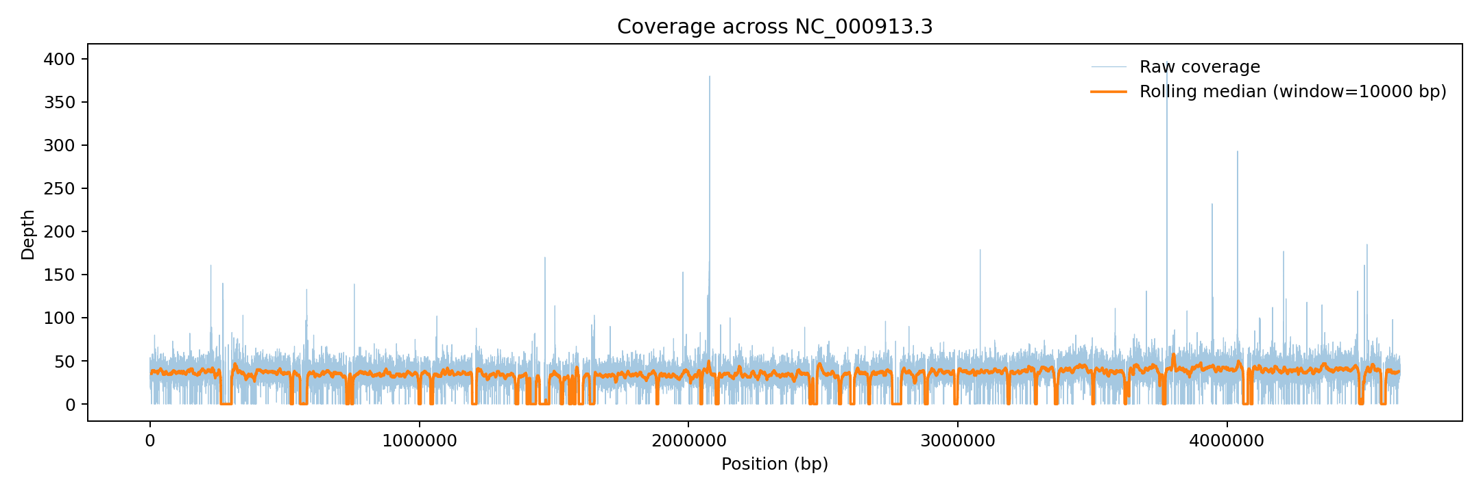
As we can see, there are many regions where both the raw depth and the sliding window of 10000 bp drop down to a depth of coverage of 0x, meaning the MG1655 strain was not the best reference genome for our analysis.

Step 6: Variant Calling

Note: To complete the tutorial on reference-based assemblies, we will assume that our alignment metrics looked good and our reference genome was a good fit.

Once we have our aligned reads in a sorted BAM file, the next step is to call variants, which means we are trying to identify the positions where our sample’s genome differs from the MG1655 reference. These differences can be:

SNPs (single nucleotide polymorphisms): A > T
MNPs (multiple nucleotide polymorphisms): CC > GT
Indels (insertions or deletions): A > ATGG or ACGA > A
Complex substitution: ACT > TCGA
Larger structural variants (> 50 bp)

Here we’ll use FreeBayes, a widely used haplotype-based variant caller for short variants. Unlike simple pileup-based approaches, FreeBayes considers read context to make more accurate calls, especially around indels.

freebayes -f MG1655.fasta VREC1013_MG1655.sorted.bam > VREC1013_MG1655.freebayes.vcf

Note: FreeBayes has many advanced options (ploidy, minimum coverage, region targeting), but the defaults are a good starting point for bacterial genomes.

Once you have your VCF file, you can generate a quick statistics report:

bcftools stats VREC1013_MG1655.freebayes.vcf | grep '^SN' > reports_stats/vcf_stats.txt

After running variant calling and summarizing our results, we obtain the following breakdown of variant types:

Variant Type	Count
Total records	86,963
SNPs	71,842
MNPs	14,363
Indels	519
Complex	317

It’s clear from the large number of reported variants that MG1655 was not an ideal reference genome for this sample, highlighting how reference choice can strongly influence the results.

Note: You may notice that the Total records doesn’t exactly equal the sum of SNPs, MNPs, Indels, and Complex variants. That’s because bcftools stats counts records and alleles differently. At multiallelic sites (positions with more than one alternate allele), a single record can contribute to multiple variant categories. So the allele-based counts are often slightly higher than the record total. This is expected and not an error.

Why are variants important?

Variants are the genetic “fingerprints” that make one strain different from another. In the context of E. coli and other bacteria, they matter because:

Tracking evolution and outbreaks: SNPs provide high-resolution markers to distinguish closely related isolates. Public health labs use variant patterns to trace foodborne outbreaks and hospital-acquired infections.
Understanding antimicrobial resistance (AMR): Many resistance phenotypes come from specific point mutations (ex: gyrA for fluoroquinolone resistance) or insertions/deletions that alter protein function. Variant calling helps identify these changes.
Identifying virulence factors: Pathogenic strains often differ from harmless lab strains by a handful of mutations or indels in key genes (ex: toxin production).
Comparing against a reference: By calling variants relative to a well-studied genome like MG1655, we can quantify how “far” our isolate is from the lab strain and highlight unique features like plasmids or genomic islands.
Building phylogenies: Sets of SNPs are used to build phylogenetic trees, showing evolutionary relationships between isolates.

In short, variants are how we connect sequence data to biology. They help us explain differences in resistance, virulence, and evolutionary history.

Tip: A useful method to validate variants is to load both your VCF file and BAM file into IGV (Integrative Genomics Viewer) to see exactly where variants occur and how well they’re supported by the reads. We will tackle this process in a later post.

Final Results

Most of the genome aligns: It’s definitely E. coli but we are not using the correct strain.
Thousands of variants appear: Extra evidence that it’s most likely not MG1655.
Some regions have no coverage: These represent regions that our strain is missing.
Some reads aren’t mapping to the reference: These represent plasmids or genomic islands that MG1655 doesn’t have and that could contain pathogenic genes.

Key Takeaways

The big lesson: reference mapping is fast and efficient when a good reference exists. It can be informative but it only shows you what’s present in the reference. Anything unique to your isolate will be invisible in this analysis.

What’s Coming Next

In the next post, we’ll take a different approach: de novo assemblies.

Instead of squeezing our sample’s genome into the framework of MG1655, we’ll assemble the genome directly from the reads themselves. This will give us a much more accurate representation of the exact strain we sequenced, including plasmids and accessory regions that were missing from the MG1655 reference.

Share on

X Facebook LinkedIn Bluesky

Mario F. Bisconti